$$\dist{x}{y}:=\left|x-y\right|=\sqrt{\sum_{i=1}^n (x_i-y_i)^2 }$$
A
sphere with radius $r$ and center $C$ is by definition the set of all the points that is
$r$ units
away from the center $C$.
$$
\{x\in \R^n: \dist{x}{C}=r\}= \{x\in \R^n: \sum_{i=1}^n (x_i-c_i)^2=r^2\}
$$
In particular, if the center is the origin $\vc{0}$, for brevity, the sphere can also be thought as the set of
solutions to the equation
$$
\sum_{i=1}^n x_i^2=r^2
$$
-
When $n=1$, $$\mathbb{R}$$ is the set of all real numbers.
The distance between numbers $x,y$ is just the absolute value of the
difference
$$\dist{x}{y}=\left|x-y\right|$$
And the "sphere" with radius $r$ and center $c$ is just the set
$$\{c-r,c+r\}$$
which are the two endpoints of the interval $[c-r,c+r]$.
-
When $n=2$, $$\mathbb{R}^2 = \{(x,y) :x,y\in\R \}$$ is the set of all ordered pairs of real numbers.
The distance between two points $x$ and $y$
$$\dist{x}{y}=\sqrt{(x_1-x_2)^2+(y_1-y_2)^2}$$
gives the well-known Pythagorean Theorem.
The "sphere" with radius $r$ and center $c$ is the set
$$\{(x,y): (x-c_1)^2+(y-c_2)^2=r^2\}$$
which is the familiar circle.
- $$\mathbb{R}^3=\{(x, y, z) \mid x, y, z \in \mathbb{R}\}$$
Surfaces and Solids
Vectors
Vector addition and scalar multiplication turns $\mathbb{R}^n$ into a vector space over
$\mathbb{R}$.
The dot product is a bilinear map from $\mathbb{R}^n\times\mathbb{R}^n$ to $\mathbb{R}$, and the cross product is
only defined for $\mathbb{R}^3$. We will discuss these in more detail in the next sections.
Unit Vectors
A unit vector is a vector with length $1$.
The following are the
standard basis
vectors for $\mathbb{R}^3$,
$$
\mathbf{i}=\langle 1,0,0\rangle \quad \mathbf{j}=\langle 0,1,0\rangle \quad \mathbf{k}=\langle 0,0,1\rangle
$$
In a n-dimensional space, $n-1$
angles are
needed
to specify a direction.
For this reason
Unit
vectors
are often used as the more efficient way to define directions.
Given any vector, $v$ we can decompose it into a direction part and a
magnitude
part as follows:
$$\color{green} v = \overbrace{\frac{v}{\|v\|}}^{direction} \quad \overbrace{\|v\|}^{length} $$
Dot and Cross Products
Dot Product
By simple computation, we have the following properties:
If $\theta$ is the angle between the vectors
$v,w$
$$
v \cdot w=|v||w| \cos \theta
$$
Equivalently,
$$
\cos \theta=\frac{ v \cdot w}{|v||w|}
$$
It follows that, $v,w$ are perpendicular, i.e. $\theta=\pi/2$ , if and only if $$v\cdot w=0$$
By the Law of Cosines:
$$
\|\mathbf{v}-\mathbf{w}\|^2=\|\mathbf{w}\|^2+\|\mathbf{v}\|^2-2\|\mathbf{v}\|\|\mathbf{w}\| \cos \theta
$$
Now, observe that:
$$
\begin{aligned}
& \|\mathbf{v}-\mathbf{w}\|^2=(\mathbf{v}-\mathbf{w}) \cdot(\mathbf{v}-\mathbf{w}) \\
& =\mathbf{v} \cdot \mathbf{v}-2(\mathbf{v} \cdot \mathbf{w})+\mathbf{w} \cdot \mathbf{w} \\
& =\|\mathbf{v}\|^2+\|\mathbf{w}\|^2-2(\mathbf{v} \cdot \mathbf{w}) \\
&
\end{aligned}
$$
Equating these two expressions for $\|\mathbf{v}-\mathbf{w}\|^2$ gives:
$$
\begin{aligned}
\|\mathbf{w}\|^2+\|\mathbf{v}\|^2-2\|\mathbf{v}\|\|\mathbf{w}\| \cos \theta &
=\|\mathbf{v}\|^2+\|\mathbf{w}\|^2-2(\mathbf{v} \cdot \mathbf{w}) \\
-2(\|\mathbf{v}\|\|\mathbf{w}\| \cos \theta) & =-2(\mathbf{v} \cdot \mathbf{w}) \\
\|\mathbf{v}\|\|\mathbf{w}\| \cos \theta & =\mathbf{v} \cdot \mathbf{w}
\end{aligned}
$$
When $v,w$ are unit vectors then,
$$
v \cdot w=\cos \theta
$$
Which is maximized when $\theta=0$, i.e. $v=w$.
Thus the dot product is often used to measure
the
similarity between two vectors.
Projections
Scalar projection of $\mathbf{a}$ onto $\mathbf{b}$:
$$\operatorname{comp}_{\mathbf{b}}
\mathbf{a}=\underbrace{\frac{\mathbf{b}}{|\mathbf{b}|}}_{direction} \cdot \mathbf{a}$$
This essentially gives the signed length of the projection.
 $$ \operatorname{comp}_{\mathbf{b}} \mathbf{a}=\|a\|\cos(\theta) = \|\mathbf{a}\|\frac{\mathbf{a} \cdot
\mathbf{b}}{\|\mathbf{a}\|\|\mathbf{b}\|} = \frac{\mathbf{a} \cdot \mathbf{b}}{\|\mathbf{a}\|}
$$
$$ \operatorname{comp}_{\mathbf{b}} \mathbf{a}=\|a\|\cos(\theta) = \|\mathbf{a}\|\frac{\mathbf{a} \cdot
\mathbf{b}}{\|\mathbf{a}\|\|\mathbf{b}\|} = \frac{\mathbf{a} \cdot \mathbf{b}}{\|\mathbf{a}\|}
$$
Vector projection of $\mathbf{a}$ onto $\mathbf{b}:$
$$\operatorname{proj}_{\mathbf{b}}
\mathbf{a}=
\underbrace{\operatorname{comp}_{\mathbf{b}}
\mathbf{a}}_{signed \ length}\quad
\underbrace{\frac{\mathbf{b}}{|\mathbf{b}|}}_{direction}=\frac{\mathbf{b} \cdot \mathbf{a}}{|\mathbf{b}|^{2}}
\mathbf{b}$$
The first equality is more meaningful, as it gives the length-direction decomposition.
For any non-zero constant $c$
$$\operatorname{proj}_{\mathbf{cb}}
\mathbf{a}=\operatorname{proj}_{\mathbf{b}}
\mathbf{a} $$
In other words, the projection of $\mathbf{a}$ onto $\mathbf{b}$ is independent of the length of $\mathbf{b}$, only
the direction of the projection matters.
The Cross Product
Motivation
Given two vectors $u,v$, we want to find a vector $w$, that is perpendicular to both $u$ and $v$.
This can be done by solving the following equations:
$$u\cdot w = u_1w_1+u_2w_2+u_3w_3 = 0 $$
$$v\cdot w = v_1w_1+v_2w_2+v_3w_3 = 0 $$
Which implies $$(u_1v_3-u_3v_1)w_1+(u_2v_3-u_3v_2)w_2=0$$
One trivial solution is to take $$w_1=u_2v_3-u_3v_2,\ w_2 = u_3v_1-u_1v_3, \ w_3=u_1v_2-u_2v_1 $$
The solution give the cross product of $u$ and $v$.
Computational Properties
Often the above the formula is not very intuitive, and difficult to recall.
Instead, one often use the Laplace Expansion for determinants:
$$\begin{aligned}\mathbf{u} \times \mathbf{v}=\left|\begin{matrix}\mathbf{i}&\mathbf{j}&\mathbf{k}\\
u_1 & u_2 & u_3\\
v_1 & v_2 & v_3\end{matrix}\right|
&= \mathbf{i} \left|\begin{matrix} u_2&u_3\\v_2&v_3 \end{matrix} \right|-
\mathbf{j} \left|\begin{matrix} u_1&u_3\\v_1&v_3 \end{matrix} \right|+
\mathbf{k} \left|\begin{matrix} u_1&u_2\\v_1&v_2 \end{matrix}
\right|\\&=\left(u_2v_3-u_3v_2,u_3v_1-u_1v_3,u_1v_2-u_2v_1\right)\end{aligned} $$
One can check that the followings true,
If $\mathbf{a}, \mathbf{b}$, and $\mathbf{c}$ are vectors and $c$ is a scalar, then
Geometric Properties
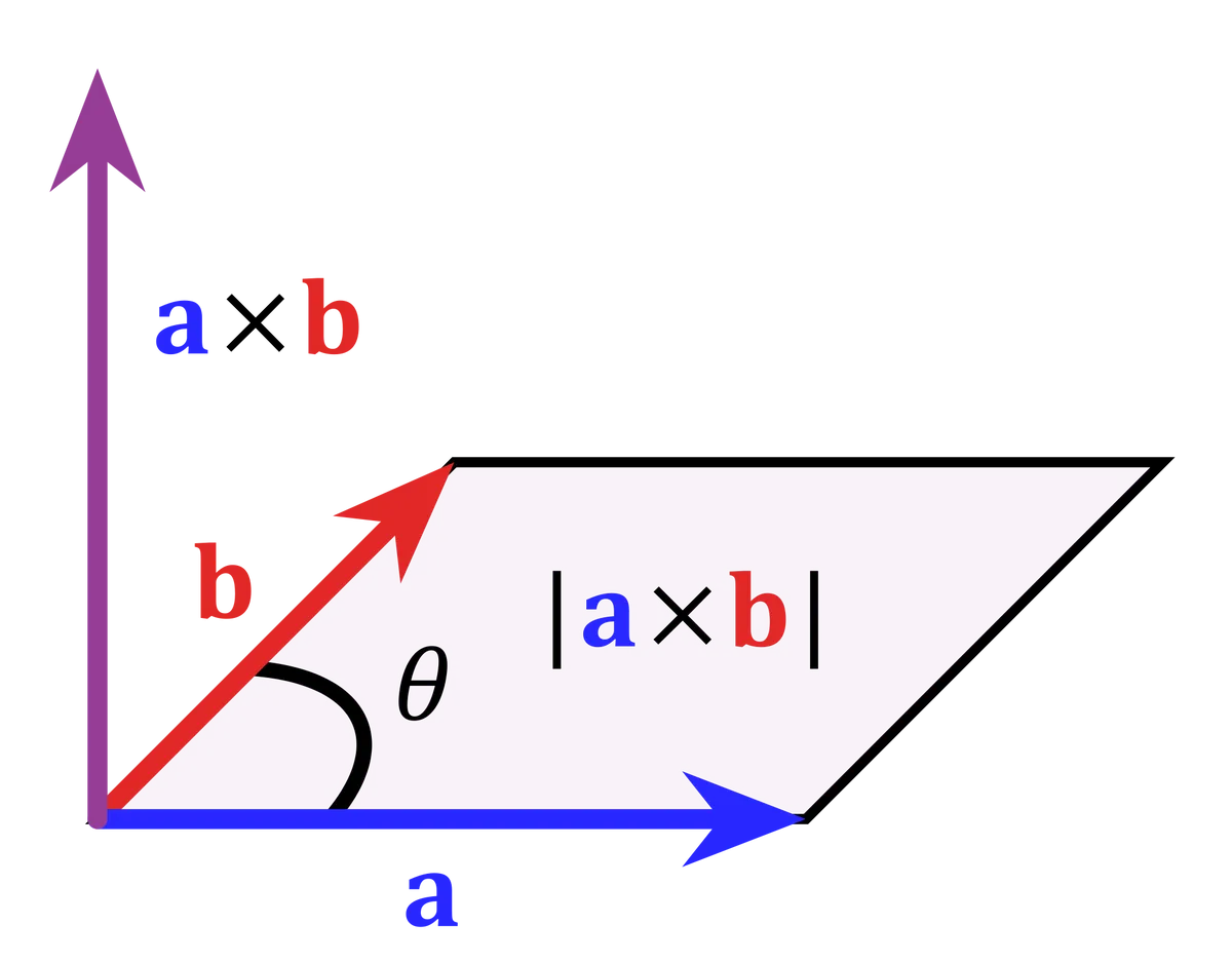
- If $\theta$ is the angle between $\mathbf{a}$ and $\mathbf{b}$, then the length of the cross product
$\mathbf{a} \times \mathbf{b}$ is given by
$$
|\mathbf{a} \times \mathbf{b}|=|\mathbf{a}||\mathbf{b}| \sin \theta
$$
And $|\mathbf{a} \times \mathbf{b}|$ gives the area of the parallelogram determined by the two vectors.
- Two nonzero vectors $\mathbf{a}$ and $\mathbf{b}$ are parallel if and only if
$$
\mathbf{a} \times \mathbf{b}=\mathbf{0}
$$
- The volume of the parallelepiped determined by the vectors $\mathbf{a},
\mathbf{b}$,
and $\mathbf{c}$ is given
by:
$$
V=|\mathbf{a} \cdot(\mathbf{b} \times \mathbf{c})|
$$
- $$
\begin{aligned}
|\mathbf{a} \times \mathbf{b}|^2
= & \left(a_1^2+a_2^2+a_3^2\right)\left(b_1^2+b_2^2+b_3^2\right)-\left(a_1 b_1+a_2 b_2+a_3 b_3\right)^2 \\
= & |\mathbf{a}|^2|\mathbf{b}|^2-(\mathbf{a} \cdot \mathbf{b})^2 \\
= & |\mathbf{a}|^2|\mathbf{b}|^2-|\mathbf{a}|^2|\mathbf{b}|^2 \cos ^2 \theta
\\
= & |\mathbf{a}|^2|\mathbf{b}|^2\left(1-\cos ^2 \theta\right) \\
= & |\mathbf{a}|^2|\mathbf{b}|^2 \sin ^2 \theta
\end{aligned}
$$
Lines and Planes
Lines
Lines can be represented in various forms
- Vector Equation :
$$r = \underbrace{r_0}_{placement}+t\underbrace{v}_{direction}$$
- Parametric Equations : $$x=x_{0}+a t \quad y=y_{0}+b t \quad z=z_{0}+c t$$
- Symmetric Equations :$$\frac{x-x_{0}}{a}=\frac{y-y_{0}}{b}=\frac{z-z_{0}}{c}$$
Line Segments
Given two points $v$ and $w$, the line segment between $v$ and $w$ can be represented by
$$r(t)=w(1-t)+vt, \qquad t\in[0,1]$$
As $t$ moves from $0$ to $1$, the point $r(t)$ moves from $w$ to $v$.
Planes
To characterize a plane, we need
- $p_0 = (x_0,y_0,z_0)$ : a point on the plane
- $n = (a,b,c)$ : a normal vector to the plane
Once we have $p_0$ and $n$, we can represent the plane in various ways
- Vector Equation :$$n \cdot \underbrace{(p-p_0)}_{\text{a vector parallel to the plane}}=0$$
- Point-Normal Form :
$$a\left(x-x_{0}\right)+b\left(y-y_{0}\right)+c\left(z-z_{0}\right)=0$$
- General Form : $$a x+b y+c z+d=0$$
-
Two planes are parallel if and only if their normal vectors are parallel.
- If two planes are not parallel, the angle between the two planes
is defined by the angle between their normal vectors.
Distances
Given plane, with point $p_0$ on the plane and normal vector $n$. Take a point $p$, the distance between $p$ and the
plane
is given by
$$D= \underbrace{|\text{comp}_{n} (p-p_0)|}_{\text{length of the projection onto normal vector $n$}} =
|\underbrace{\frac{n }{|n|}}_{unit\ normal}\cdot (p-p_0)|$$
Given the coordinates of $p = (x_1,y_1,z_1)$, and the plane has the general form $ax+by+cz+d=0$
then the distance between $p$ and the plane can be simplified to
$$D=\frac{\left|a x_{1}+b y_{1}+c z_{1}+d\right|}{\sqrt{a^{2}+b^{2}+c^{2}}}$$
Single Variable Functions
R--> R
R--> R^n
Space Curve
For vector-valued functions, we will only consider the case where the domain lives in $\mathbf{R}$, i.e. functions of
the
form
$$v(t)= \left(v_1(t),v_2(t),v_3(t)\right),\qquad t\in D \subset \mathbf{R}$$
The function $v(t)$ lives in $\mathbf{R}^4$.
For the purpose of visualizing the function, we project it onto $\mathbf{R}^3$ along the $t$-axis,
to get the
space
curve
What is the space curve for each of the following ?
- $$v(t) = (1+t,5t+2,t)$$
- $$v(t) = \cos(t) \mathbf{i}+\sin(t) \mathbf{j}+ t\mathbf{k}$$
Some familiar concepts from calculus I, can be extend easily to vector functions.
Bridge between Cal 1 and Cal 3
A typicial Calculus 1 class deal with functions of the form
$$f: \mathbb{R}\to \mathbb{R}$$
For the geometric problems in Calculus 1, it is often more convenient to view the function
as a vector function
$$v: \mathbb{R}\to \mathbb{R}^2$$
$$ x\mapsto (x,f(x))$$
And the tangent vector of $v$ at $t$
$$v'(t) = \left(1,f'(t)\right)$$ gives the direction of the tangent line for $f$ at $t$.
R^n --> R
Limits and Continuity
Contour Plot
We will be mainly deal with functions of the form
$$f: \mathbb{R}^2\to \mathbb{R}$$
The extension of most results to $f: \mathbb{R}^n\to \mathbb{R}$ is trivial.
The graph of a function $(x,y) \mapsto z$ lives in the 3 dimensional space.
One way to visualize the function without requiring too much computational power is to consider the
level
curves.
A level curve of a function $f:\mathbb{R}^2\to \mathbb{R}$ is a curve with equation
$$f(x,y)=k$$
where $k$ is a constant, the level of that particular curve.
The collection of level curves gives a
contour plot of the function.
Limits
The limit of a function $f:\R^n\to \R$ at the point $\vc{v} $ is $L$, written as
$$
\lim _{\vc{x} \rightarrow \vc{v}} f(\vc{x})=L
$$
if for every number $\varepsilon>0$ there is a corresponding number $\delta>0$ such that if $ \vc{x} \in D$,
$$0
< |\vc{x}-\vc{v}|<\delta \longrightarrow |f(\vc{x})-L|<\varepsilon$$ The function is
continuous at $\vc{v}$ if $$\lim_{\vc{x}\to \vc{v} }f(\vc{x})=f(\vc{v})$$
$$\lim f \pm \lim g = \lim (f\pm g)$$
$$\lim cf = c \lim f$$
$$\lim (f g)= (\lim f )( \lim g )$$
$$\lim (f/g)= (\lim f )/( \lim g ),\qquad \lim g \ne 0$$
Derivatives
Directional Derivatives
To talk about the
rates of change of a function with respect to a given direction, we define the
directional
derivatives.
Note that
$$ D_{\mathrm{u}} f(x, y)=f_{x}(x, y) a+f_{y}(x, y) b = (f_x,f_u)\cdot \mathrm{u}$$
This gives the motivation to define
If $f$ is a function of two variables $x$ and $y$, then the gradient of
$f$ is
the
vector function $\nabla f$ defined by
$$
\nabla f(x, y)=\left( f_{x}(x, y), f_{y}(x, y)\right)
$$
Chain Rule
Geometries
Linear Approximation
Behavior of a function near a point is approximately linear.
Gradient Ascent / Descent
- $\frac{\nabla f}{|\nabla f|}$ gives the direction that provides the the maximum directional derivative of
$f$.
- $-\frac{\nabla
f}{|\nabla f|}$ gives the direction with the minimum directional derivative of $f$.
- The gradient at $\mathbf{v}$, $\nabla f(\mathbf{v})$, is perpendicular to the level curve / surface
$f(\mathbf{x})=f(\mathbf{v})$
- Given $\mathbf{u}$ a unit vector, note that the following dot product $$D_\mathbf{u} f=\nabla f\cdot
\mathrm{u}=|\nabla f | |u| \cos \theta $$
is maximized when $\cos \theta = 1$, i.e. $u$ is in the same direction as $\nabla f$, i.e.
$$ \mathrm{u} = \frac{\nabla f}{|\nabla f|} $$
Similarly,
the dot product is minimized when $$ \mathrm{u} = -\frac{\nabla f}{|\nabla f|} $$
- Let $r(t)$ be a parametric curve living on the level surface, then $$
f(r(t))=f(\mathbf{v})$$ using Chain rule
$$f_{1} \frac{dx_1}{dt}+\cdots+f_{n} \frac{dx_n}{dt}=\nabla f \cdot r'(t)=0$$
A physical intepretation : The level surfaces can be view as a stable planes, the
best direction to "jump toward" in order to escape the gravity of the stable planes is the perpendicular
direction.
And this is the direction of the gradient, since it is perpendicular to the stable plane.
Optimization
Derivative Tests
First Derivative
If
-
$f$ has a local maximum or minimum at $(a, b)$
- and the
first-order
partial derivatives of $f$,
exist
then $$f_{x}(a, b)=f_{y}(a, b)=0$$
The conditions $f_{x}(a, b)=0$ and $f_{y}(a, b)=0$ essentially implies that
$$D_u f(a,b) =0 \qquad \forall u$$
Second Derivative
Suppose
- the second partial derivatives of $f$ are
continuous on a
disk with center $(a, b)$,
- and that $f_{x}(a, b)=0$ and $f_{y}(a, b)=0$ .
Let
$$
D=D(a, b)=f_{x x}(a, b) f_{y y}(a, b)-\left[f_{x y}(a, b)\right]^{2}
$$
- If $D>0$ and $f_{x x}(a, b)>0$, then $f(a, b)$ is a local minimum.
- If $D>0$ and $f_{x x}(a, b)<0$, then $f(a, b)$ is a local maximum.
- If $D<0$, then $(a, b)$ is a saddle point of $f$.
- If $D = 0$, it could be a local min / max or a saddle point.
We will prove the more general case of $f: \mathbb{R}^n \to \mathbb{R}$, and this will follow as a special
case.
In the more general case of $f: \mathbb{R}^n \to \mathbb{R}$, the second derivative test can be generalized.
The
Hessian
$H_f$ of $f: \mathbb{R}^n \to \mathbb{R}$ is the matrix of second partial derivatives of $f$, more
explicitly
$$(H_f)_{ij}=f_{x_i}f_{x_j} $$
A matrix $A$ is
postive semidefinite
if $$
x^TAx \substack{>\\ {\color{red}\mathbf{\_}}} 0 \quad \forall x
$$
or equivalently
$$
Ax=\lambda x \implies \lambda \substack{>\\ {\color{red}\mathbf{\_}}} 0
$$
negative semidefinite
are defined similarly.
Let $f(x):\mathbb{R}^n\to\mathbb{R} $,
if $f\in C^2$, then at a critical point $x_0$,
- if $H_f(x_0)$ is positive definite , then $x_0$ is a local minimum,
- if
$H_f(x_0)$ is negative definite, then $x$ is a local maximum,
- otherwise, $x_0$ is point is saddle point.
$$ \begin{aligned}
y=f(\mathbf{x}+\Delta \mathbf{x}) = f(\mathbf{x})+\nabla f(\mathbf{x})^{\mathrm{T}} \Delta
\mathbf{x}+\frac{1}{2} \Delta \mathbf{x}^{\mathrm{T}} \mathbf{H}(\mathbf{x}) \Delta \mathbf{x} + \O{\|\Delta
\mathbf{x}\|^{3}}
\end{aligned}$$
- If $x_0$ is a critical point, then for $f(x_0+\Delta \mathbf{x}) $, $\nabla f(x_0)=0$
-
and $\mathbf{H}(x_0)$ is positive definite implies $$\Delta \mathbf{x}^{\mathrm{T}} \mathbf{H}(\mathbf{x})
\Delta \mathbf{x}>0$$ for all $\Delta \mathbf{x}\ne \vec{0}$
Global optimum
To guarantee global global optimum, we can either impose a boundedness condition on the domain, or require
that the function is convex / concave.
If $f$ is continuous on a closed, bounded set $D$ in $\mathbb{R}^{2}$.
Then there exists a point $\left(x_{0}, y_{0}\right)$ in $D$ such that
$$ f(x_0,y_0) \le f(x,y) \quad \forall (x,y) \in D$$
and there exists a point $\left(x_{1}, y_{1}\right)$ in $D$ such that
$$ f(x_1,y_1) \ge f(x,y) \quad \forall (x,y) \in D$$
A function $f:\mathbb{R}^n\to\mathbb{R}$ is
-
convex if $H_f(x)$ is positive definite for all $x\in\mathbb{R}^n$.
-
concave if $H_f(x)$ is negative definite for all $x\in\mathbb{R}^n$.
-
If $f$ is convex, then $f$ has a unique global maximum.
-
If $f$ is concave, then $f$ has a unique global minimum.
Lagrange Multipliers
To optimize $f(x,y,z)$ with constraints $g(x,y,z)=k$, assuming
-
absolute minimum / maximum exist
- $\nabla g\ne
0$ on on $g(x,y,z)=k$
The absolute minimum / maximum of $f$ is achieved at some points $(x,y,z)$ in the solution set of
$$\begin{aligned}
\nabla f(x, y, z) &=\lambda \nabla g(x, y, z) \\
g(x, y, z) &=k
\end{aligned}$$
Consider optimizing the function on curves in the space defined by the constraints.
-
Let $(x_0,y_0,z_0)$ be a critical on the constraints surface.
-
Let $r(t)$ any curve on the surface that passes through $(x_0,y_0,z_0)$ at $t=0$.
Then
$$
\nabla f(r(0)) = \nabla f(r(0)) \cdot r'(0) = 0
$$
-
This show that $\nabla f$ is orthogonal to the constraints surface at critical points.
-
And we know $\nabla g$ is orthogonal to the constraints surface at all points on the surface.
thus $\nabla f$ is parallel to $\nabla g$ at
critical points, i.e.
$$
\nabla f = \lambda \nabla g
$$
The effect of constraints $$g(x,y,z)=k$$
is essentially narrowing the domain of $f$ to the solution set of the above equation.
Thus, the problem is really just optimization $f$ within the restricted domain.
If $$g(x,y,z) = (\sqrt{x^2+y^2}-4)^2 + z^2 = 1 $$
Then the problem becomes optimizing $f$ on the surface of a torus.
Integration
Double and Triple Integrals
Let $D$ be a region in $\mathbb{R}^{2}$, and let $f$ be a function defined on $D$.
The
double integral
of $f$ over $D$ is defined as
$$
\begin{aligned}
\int_{D} f(x, y) d A&= \lim_{n,m \to \infty} \sum_{i=1}^{n} \sum_{j=1}^{m} f\left(x_{i, j}, y_{i, j}\right)
\Delta
A_{i, j} \\
\int_{D} f(x, y)\ dx\ dy&= \lim_{n \to \infty} \sum_{i=1}^{n}\left( \lim_{m \to \infty} \sum_{j=1}^{m}
f\left(x_{i, j}, y_{i,
j}\right)\ \Delta x_{i, j} \right) \Delta y_{i, j} \\
\end{aligned}
$$
where
- $\{A_{i,j} \}$ is a minimum cover of
the region $D$ by $n*m$ rectangles of equal length and width
-
$(x_{i, j}, y_{i, j})$ is the midpoint of $A_{i, j}$,
-
$\Delta A_{i, j}$ is the area of the rectangle with midpoint $(x_{i, j}, y_{i, j})$,
Triple and higher order integrals are defined similarly.
The Fubini's Theorem allows us to switch the order of integration.
If $f$ is continuous on the rectangle
$$
R=\{(x, y) \mid a \leqslant x \leqslant b, c \leqslant y \leqslant d\}
$$
then
$$
\iint_{R} f(x, y) d A=\int_{a}^{b} \int_{c}^{d} f(x, y) d y d x=\int_{c}^{d} \int_{a}^{b} f(x, y) d x d y
$$
Change of Variables
Polar
$$
x=r \cos \theta \quad y=r \sin \theta
$$
$$
r^{2}=x^{2}+y^{2} \quad \theta=\tan^{-1} \frac{y}{x}
$$
If $f$ is continuous on a polar rectangle $R$ given by $$0 \leqslant a \leqslant r \leqslant b, \alpha
\leqslant
\theta \leqslant \beta$$ where $0 \leqslant \beta-\alpha \leqslant 2 \pi$, then
$$
\iint_{R} f(x, y) d A=\int_{\alpha}^{\beta} \int_{a}^{b} f(r \cos \theta, r \sin \theta) r d r d \theta
$$
Cylindrical
$$
x=r \cos \theta \quad y=r \sin \theta \quad z=z
$$
$$
r^{2}=x^{2}+y^{2} \quad \tan \theta=\frac{y}{x} \quad z=z
$$
Suppose that $f$ is continuous on
$$
E=\left\{(x, y, z) \mid(x, y) \in D, u_{1}(x, y) \leqslant z \leqslant u_{2}(x, y)\right\}
$$
where $D$ is given in polar coordinates by
$$
D=\left\{(r, \theta) \mid \alpha \leqslant \theta \leqslant \beta, h_{1}(\theta) \leqslant r \leqslant
h_{2}(\theta)\right\}
$$
Then $$\iiint_{E} f(x, y, z) d V=\int_{\alpha}^{\beta} \int_{h_{1}(\theta)}^{h_{2}(\theta)} \int_{u_{1}(r \cos
\theta, r \sin \theta)}^{u_{2}(r \cos \theta, r \sin \theta)} f(r \cos \theta, r \sin \theta, z) r d z d r d
\theta$$
Spherical
$$(\rho, \theta,\phi)\to \begin{cases}z&=\rho \cos(\phi)\\
\underbrace{r}_{shadow}&=\rho\sin(\phi) \end{cases}\to \begin{cases}
z&=\rho \cos(\phi) \\
y&=\rho\sin(\phi)\sin(\theta)\\
x&=\rho\sin(\phi)\cos(\theta) \end{cases}$$
Where $\rho^2=x^2+y^2+z^2$
If $f$ is continuous on $$
E=\{(\rho, \theta, \phi) \mid a \leqslant \rho \leqslant b, \alpha \leqslant \theta \leqslant \beta, c
\leqslant
\phi \leqslant d\}
$$then
$$ \iiint_{E} f(x, y, z) d V
=\int_{c}^{d} \int_{\alpha}^{\beta} \int_{a}^{b} f(\rho \sin \phi \cos \theta, \rho \sin \phi \sin \theta,
\rho
\cos
\phi) \rho^{2} \sin \phi d \rho d \theta d \phi
$$
All of these transformations are essentially special cases of the change of variables
theorem. We will cover the general case
in the next section, where we introduce the Jacobian and Jacobian
determinant.
Vector Calculus
R^n --> R^m
Jacobian and Change of Variables
Let $f:\R^n\to\R^m$ be a differentiable function. The Jacobian matrix of $f$ is the
matrix
$$
J_f= \begin{pmatrix}
\frac{\partial f_1}{\partial x_1} & \cdots & \frac{\partial f_1}{\partial x_n}\\
\vdots & \ddots & \vdots\\
\frac{\partial f_m}{\partial x_1} & \cdots & \frac{\partial f_m}{\partial x_n}
\end{pmatrix}
$$
The Jacobian determinant of $f$ is the determinant of the Jacobian matrix
$$
\det J_f$$
For simplicity, the notation $$\dfrac{\partial f}{\partial x}=J_f$$ will also be used.
Chain Rule :
If $f: \R^n \to \R^m$ and $g: \R^m \to \R^w$ are differentiable, then
for $$h:\mathbf{v}\mapsto g(f(\mathbf{v}))$$
$$ J_h(\mathbf{v})=
J_g(f(\mathbf{v})) J_f(\mathbf{v}) $$
- If $f:\R^2\to\R^2$ is given by $f(r, \theta)=(r \cos \theta, r \sin \theta)$, then
$$
J_f=\begin{pmatrix}
\cos \theta & -r \sin \theta\\
\sin \theta & r \cos \theta
\end{pmatrix} , \qquad \det J_f=r
$$
-
If $g:\R^2\to\R^2$ is given by $g(x, y)=(\sqrt{x^2+y^2}, \tan^{-1}(y/x))$, then
$$
J_g=\begin{pmatrix}
\frac{x}{\sqrt{x^2+y^2}} & \frac{y}{\sqrt{x^2+y^2}}\\
-\frac{y}{x^2+y^2} & \frac{x}{x^2+y^2}
\end{pmatrix} , \qquad \det J_g= \frac{1}{\sqrt{x^2+y^2}}
$$
Let
-
$T(\vc{v})=\vc{x}$ be differentiable and injective,
-
$T$ maps a region $D$ to a region $D'$,
- If $F\in C[D]$ is continous
then
$$\int_D F(\vc{x}) d\vc{x}=\int_{D'} F(T(\vc{v})) |\det J_T(\vc{v})| d\vc{v}$$
If
- $f\in C[R^n]$
- $f(p)\ne 0$
then there exist an open set $U$ containing $p$ such that, on $U$
- $f$ is invertible
-
$$J_{f^-1} = (J_f)^{-1}$$
Vector Fields
A vector field is a map $$F:\R^n\to\R^n$$
If a vector $F=\nabla f$ for some scalar function $f$, $F$ is called a conservative vector
field.
For $f:\R^n\to \R$, the following map defines a vector field
$$F:\mathbf{v}\mapsto \nabla f(\mathbf{v})$$
Operators on Vector Field
The divergence of a vector field $F$ is the scalar
function
$$\operatorname{div} F = \nabla \cdot F $$
The curl of a vector field $F$ is the vector function
$$\operatorname{curl} F = \nabla \times F $$
- If $f\in C^2[\R^3]$, then
$$
\operatorname{curl}(\nabla f)=\mathbf{0}
$$
- If $\mathbf{F}\in C^1(\R^3,\R^3)$
and curl $\mathbf{F}=\mathbf{0}$, then $\mathbf{F}$ is a conservative vector
field.
-
If $\mathbf{F}\in C^2(\R^3,\R^3)$, then
$$
\operatorname{div} \operatorname{curl} \mathbf{F}=0
$$
Path Integral
Path Integral for real-valued functions
If $f$ is defined on a smooth curve $C$ given by $$x=x(t),\qquad y=y(t),\qquad t\in [a,b]$$
the path integral of $f$ along $C$ is defined by the following limit (if it exist)$$\int_{C} f(x,
y) d s=\lim _{n \rightarrow \infty} \sum_{i=1}^{n} f\left(x_{i}^{*}, y_{i}^{*}\right) \Delta s_{i}$$
If $f$ is continuous on the smooth curve $C$, and $r(t),\ t\in [0,1]$ is a parametrization of $C$,
then
$$\begin{aligned}
\int_{C} f(x, y) d s&= \int_0^1 f(r(t)) \underbrace{|r'(t)| \ dt}_{ds}\\
&=\int_{0}^{1} f(x(t), y(t)) \sqrt{\left(\frac{d x}{d t}\right)^{2}+\left(\frac{d y}{d
t}\right)^{2}} d t
\end{aligned}$$
Path Integral for Vector Fields
We will assume $\mathbf{F}$ is a continuous vector field defined on a smooth curve $C$ given by a vector function
$\mathbf{r}(t), a \leqslant t \leqslant b$.
The path integral of
$\mathbf{F}$
along $C$ is
$$
\int_{C} \mathbf{F} \cdot d \mathbf{r}=\int_{a}^{b} \mathbf{F}(\mathbf{r}(t)) \cdot \mathbf{r}^{\prime}(t) d
t
$$
If $ \mathbf{F} =\nabla f$ for some function $f$, then
$$\mathbf{F}(\mathbf{r}(t)) \cdot \mathbf{r}^{\prime}(t)=\nabla f(\mathbf{r}(t)) \cdot
\mathbf{r}^{\prime}(t)$$
is
essentially the rate of change of $f$ at time $t$ when travel along the path.
If $\mathbf{F}=P \mathbf{i}+Q \mathbf{j}$, then
$$
\begin{aligned}
\int_{C} \mathbf{F} \cdot d \mathbf{r}&=\int_{a}^{b} \mathbf{F}(\mathbf{r}(t)) \cdot \mathbf{r}^{\prime}(t) d
t& \color{blue} =\int_{a}^{b} \mathbf{F}(\mathbf{r}(t)) \cdot \underbrace{\mathbf{T}}_{\frac{r'(t)}{|r'(t)|}}\
\underbrace{ds}_{|r'(t)|dt}
\\
&=\int_{a}^{b} P(x,y) x'(t) dt + Q(x,y) y'(t) dt\\
&=\int_{C}P(x,y) dx + Q(x,y) dy
\end{aligned}
$$
If $P_y=Q_x$, then $F$ is conservative.
If $F$ is conservative, and $C$ is a smooth curve with initial point $A$ and terminal point $B$, then
$$\int_{C} \mathbf{F} \cdot d \mathbf{r}= f(B)-f(A)$$
Green's Theorem
If $C$ is positively oriented, piecewise-smooth, simple closed curve in the plane, then
$$
\int_{C} \mathbf{F} \cdot d \mathbf{r}= \iint_D (Q_x - P_y) d A
$$
The Green's Theorem is a special case of Stokes' Theorem.
Surface Integral
\begin{aligned}
\iint_{S} f(x, y, z) d S&=\lim _{m, n \rightarrow \infty} \sum_{i=1}^{m} \sum_{j=1}^{n} f\left(P_{i
j}^{*}\right)
\Delta S_{i j}\\
&=\iint_{D} f(\mathbf{r}(u, v))\left|\mathbf{r}_{u} \times \mathbf{r}_{v}\right| d A
\end{aligned}
We will assume $\mathbf{F}$ is a continuous vector field defined on a smooth oriented surface $S$ with unit normal
vector $\vc{n}$.
The surface integral of $\mathbf{F}$ over $S$ is
$$
\iint_{S} \mathbf{F} \cdot d \mathbf{S}=\iint_{S} \mathbf{F} \cdot \mathbf{n} d S=\iint_{D} \mathbf{F}
\cdot\left(\mathbf{r}_{u} \times \mathbf{r}_{v}\right) d A
$$
This integral is also called the flux of $\mathbf{F}$ across $S$.
If $C$ the a positively oriented, piecewise-smooth, simple closed boundary curve of $S$, then
$$ \int_{C} \mathbf{F} \cdot d \mathbf{r}= \iint_{S} \text{curl } \mathbf{F} \cdot d \mathbf{S}$$
Geometry of divergence and curl
$$
\left.\operatorname{div} \mathbf{F}\right|_{\mathrm{x}_0}=\lim _{V(S) \rightarrow 0} \frac{1}{V(S)} \iint_{S}
\mathbf{F} \cdot \hat{\mathbf{n}} d S = \text{net flow out (+) or in (-) of } x_0
$$
$$
\left.\operatorname{curl} \mathbf{F}\right|_{\mathrm{x}_0}=\lim _{A(C)\rightarrow 0} \frac{1}{A(C)} \oint_{C}
\mathbf{F} \cdot d \mathbf{r} = \text{net circulation around } x_0
$$
Complex Analysis
$$\begin{aligned}
z&=r(\cos \theta + i \sin \theta) \quad &&\color{green}\text{Euler's Formula}\\
&= r e^{i \theta} \quad &&\color{green}\text{Polar Form}
\end{aligned}$$
Functions $$f: \C\to C$$
$$f(x+iy)=u+vi$$
can be viewed as functions of the form
$$f':\R^2\to \R^2$$
$$(x,y)\mapsto (u(x,y),v(x,y))$$
Functions
-
$$z\mapsto z^n=:w\qquad n\in \Z - \{0\}$$
$$|w|=|z|^n$$
$$\arg{w}=
\begin{cases}
n\arg{z} & n>0\\
n^{-1}\arg{z} & n<0 \end{cases} $$
-
$$z\mapsto \sqrt{z}=:w$$
$$|w|=|z|^{1/2}$$
$$\arg(w)=\frac{1}{2}\Arg{z}$$
-
$$z\mapsto e^z=:w$$
$$|w|=e^{|z|}$$
$$\arg(w)=\arg(z)$$
-
$$z\mapsto \Log{z}$$
$$|w|= \log |z|$$
$$\arg(w)=\Arg z$$
-
$$
\begin{aligned}
& \cos z=\frac{e^{i z}+e^{-i z}}{2}, \quad z \in \mathbb{C} \\
& \sin z=\frac{e^{i z}-e^{-i z}}{2 i}, \quad z \in \mathbb{C} \\
&
\end{aligned}
$$
-
$$
\begin{aligned}
& \cosh z=\frac{e^z+e^{-z}}{2}, \quad z \in \mathbb{C} \\
& \sinh z=\frac{e^z-e^{-z}}{2}, \quad z \in \mathbb{C} \\
&
\end{aligned}
$$
$$e^z:= \sum_{n=0}^{\infty} \frac{z^n}{n!}$$
Differentiation
Integration
Let $f:\C \to \C$ be holomorphic on a simply connected domain $U$.
Then
$$\oint_{C} f(z) dz= 0 $$
for any closed curve $C$ in $U$.
This is a corollary follows from Green's Theorem .
$$
\begin{aligned}
\oint_{C} f(z) dz&=\oint_{C} \left(u+iv\right) dz\\
&=\oint_{C} (u+iv) (dx+idy )\\
&=\oint_{C} (u+iv) dx+ (iu-v) dy\\
&=\iint_D (iu_x-v_x)- (u_y+iv_y) dA \qquad \color{green}\text{Green's Theorem}\\
&=\iint_D 0 dA \qquad \color{red}\text{Cauchy Reimann Eqs}\\
&=0
\end{aligned}
$$
- Let $f:U \to \C$ be holomorphic on a open subset $U\subset \C$.
-
Let $D$ be a open disk in $U$ with boundary $\gamma$.
Then
$$
f^{(n)}(a) = \frac{n!}{2\pi i} \oint_{\gamma} \frac{f(z)}{(z-a)^n} dz
,\qquad \forall a\in D
$$
Measure Theory
Measurable
Measurable Spaces
A $\sigma$-field on $X$ is a collection
$$
\mc{A}\subseteq 2^X
$$
that satisfies the following properties:
-
$X \in \mc{A}$
-
If $A\in \mc{A}$, then $A^c \in \mc{A}$
-
If $A_1, A_2, \dots \in \mc{A}$, then $\bigcup_{n=1}^{\infty} A_n \in \mc{A}$
$(X, \mc{A})$ is called a measurable space.
If $\mc{A} \subset 2^X$ is a $\sigma$-field, then
-
$\emptyset \in \mc{A}$
-
If $A_n \in \mc{A}$ for all integers $n$, then $\bigcap_{\N} A_n \in \mc{A}$
-
If $X$ is a finite set, then all of the following are $\sigma$-fields:
$$\{
\emptyset, X
\}$$
$$2^X$$
$$\{
\emptyset, X, \{x\}, X\setminus \{x\}
\}\qquad x\in X $$
-
Let $S\subset 2^X$, the
$\sigma$-field generated by $S$
$$\sigma(S)$$ is
the smallest $\sigma$-field containing $S$.
If $(X,\tau)$ is a topological space,
$$\sigma(\tau)$$
is called the Borel $\sigma$-field on $X$.
Measures
A measure on a measurable space $(X,\mc{A})$ is a function
$$
\mu: \mc{A} \to [0,\infty]
$$
that satisfies the following properties:
-
$\mu(\emptyset)=0$
-
$\{A_1\}\in \mc{A} \implies \mu(\bigcup_{n=1}^{\infty} A_n) = \sum_{n=1}^{\infty} \mu(A_n)$
- Counting Measure
Let $X$ be a finite set, then
$$
\mu(A) = |A|
$$
is a measure on $(X,2^X)$.
-
Point Measure
-
Let $x_1, x_2, \dots \in X$ be a sequence of distinct points,
-
and $a_1, a_2, \dots \in \R^{\ge 0}$.
$$
\mu(A) = \sum_{i=1}^{\infty} a_i \delta_{x_i}(A) = \sum_{i=1}^{\infty} a_i 1_{A}(x_i)
$$
-
Lebesgue Measure
On $(\R, \mc{B}(\R))$, the Lebesgue measure is the unique measure such that
$$
\mu([a,b]) = b-a
$$
Measurable Maps
A measurable map $f: (X,\mc{A}) \to (Y,\mc{B})$ is a function
$$
f: X \to Y
$$
such that
$$
f^{-1}(B) \in \mc{A}
$$
for all $B\in \mc{B}$.
-
Given $X, Y$ topological spaces with respective Borel $\sigma$-fields.
Then any continuous map $f: X \to Y$ is measurable.
-
If $(f_n)$ are measurable maps $E\to \bar{R}$, then
$$
\sup_{\N} f_n,\ \inf_{\N} f_n,\ \limsup_{n\to\infty} f_n,\ \liminf_{n\to\infty} f_n
$$
are measurable maps.
Integration
Simple Functions
A function $f: X \to \bar{\R}$ is called a simple function if
$$
f(X) = \{a_1, a_2, \dots, a_n\}
$$
for some $a_1, a_2, \dots, a_n \in \R$.
The integral of a simple function $f$ is defined as
$$
\int_X f d\mu = \sum_{i=1}^{n} a_i \mu(f^{-1}(a_i))
$$